Visualizing and Refining a Terrain Survey

Introduction:  The development of geospatial information systems (GIS) has allowed new avenues and research methods to be created that help evaluate spatial questions and problems. Digital Surface modeling is one improved method for those evaluations. In a GIS, there are many ways in which a dataset of elevation values can be reviewed to create a digital representation of a real world surface. This exercise explores several options on how to create a continuous surface from a point feature class using ArcGIS software.

Inverse Distance Weighted Interpolation (IDW): Inverse distance weighted interpolation (IDW) uses the concept of areas that are closer together have more in common than those that are a farther distance apart. To help model a surface from a set of elevation data points, IDW will use a defined search area, use all the elevation points that fall within the area, apply a weight based on distance from the area being modeled, and assign a value to the surface based on the average in that search area. If the dataset used in the interpolation has a large number of survey points at a fine resolution, IDW is a great method to use; however, because there is no standard and uses average values, the results can’t be conclusive that the surface represents the real world features correctly.

Natural Neighbor: A natural neighbor interpolation of a surface uses surrounding survey points similar to IDW but instead of distance, uses a proportion of areas of overlap. The creation of Thiessen Polygons around the survey points is the first step this process runs, then using the point where the surface is being calculated, another Thiessen polygon is created overlapping the originals. Using the proportion of the overlapped original polygons to the newly created polygon, weights are applied to the surrounding survey values and used to assign a surface value at the point in question. This is better suited for datasets that have fewer survey points that are low density of the study area. 

Spline: Using a spline to create a continuous surface from a point feature class is capable from a statistical equation figured from the dataset. The surface created tries to minimize the variation among values resulting in a very smooth surface model. This is great for areas of little variance, but for formations that have drastic changes in elevation, features may be represented falsely in the digital model. Spline is a “connect the dots” form of interpolation where each elevation point is plotted at its observed value and the created digital surface passes through each recorded point like a sheet to form a continuous model.

Kriging: Kriging, unlike the spline or IDW modes of interpolation, uses a statistical model created from the survey data and applies it to the model to create a surface. Since a statistical model is used to create the surface, a degree of certainty can be calculated allowing for an accuracy of a surface model to be evaluated more directly as compared to the surface estimations created by a IDW or spline. Like IDW, Kriging interpolation weights surrounding values and applies the results to an area that doesn't have surveyed values. The weight assigned to each value is based on distance to the point in question as well as the overall arrangement of all survey points in a study area. This takes the whole area into consideration but still allows the “closer areas are more similar” idea to persist in the model. Like an IDW, Kriging interpolation is more accurate with higher numbers of original survey data points; however, Kriging interpolation can also be a reliable method for surface modeling with few data points if the survey points are accurate and reflected accordingly in the statistical model generated for that dataset.

Triangular Irregular Network(TIN): A triangular irregular network (TIN) is created from a point feature class by connecting neighboring survey points. The connection of these points creates triangles that allows the surface to shape and follow the grades of the terrain. A TIN can be used to create a 3D representation of a surface to provide the GIS user a better visual representation of a study area. When using a TIN, areas that have more variance in elevation should have more reference points to allow the triangles to better conform to the feature. If an area is surveyed at a coarse scale, subtle changes in topography may be lost by the generalization of the triangles created.

Methods:

Figure 1: Formatted in the previous exercise, the XYZ coordinates for the terrain were imported into a Microsoft Excel table. To remove the negative Z values and keep the scale of the surface true, a value of 12 was added to all X, Y, and Z recordings. 

Importing the Elevation Data: Before any terrains can be created in ArcMap, the XYZ table of values created in the last exercise needs to be imported into ArcGIS (Figure 1). The table should be saved in a geodatabase or file accessible by ArcMap, if not available, the table won’t be visible to the program. Once the table is saved in the appropriate space, right click “Layers” under the table of contents. From the menu, click “Add Data”. Browse the folders in the window to find the saved table of coordinates then click and add the file to the map. At this point, the chart is only a table and is not a feature class in ArcMap. To display the coordinates in the map view, right click the table in the table of contents and from the drop down menu select “display XY Data”. Make sure that the X, Y, and Z values are assigned correctly to correctly display the coordinates. Now the coordinates are displayed as points on the map viewer. Switch the table of contents to the “list by drawing order” view to hide the original table. The point feature class should be the only item displayed in the table of contents. The feature class now needs to be exported. It is important to EXPORT the XY display to a new feature class and not just save. By exporting the features, ArcGIS saves all the information and the relative associations by assigning object IDs to each set of coordinates. These associations are what the tools will read and use as references in later processes. Right click the point feature class and from the menu select “Data-Export Data” and follow the prompts to save the new feature class to a geodatabase. The saved feature class will then be added to the table of contents and is now able to be used by other ArcGIS tools.    

Figure 2: ArcGIS offers an extensive list of tools and operations. For the surface interpolations done in this exercise, all the tools with the exception of a TIN are located in the 3D Analyst Tools toolbox under the Raster Interpolation toolset. 

IDW Interpolation: The inverse distance weighted (IDW) interpolation is performed by running the IDW tool from the ArcGIS toolbox (Figure 2). To run the tool, open ArcToolbox and expand the “3D analysis tools” toolset. From the “Raster Interpolation” toolset, select “IDW”. The IDW tool window will open. Use the coordinate point feature class as the “input features”. Make sure to select the Z field as the “Z value field” to make sure the tool uses the elevation values in the interpolation. Name the output raster, accept the defaults, and select OK to run the interpolation.

Natural Neighbor Interpolation: The natural neighbor interpolation is performed by running the “natural neighbor” tool from the ArcGIS toolbox (Figure 2). To run the tool, open ArcToolbox and expand the “3D analysis tools” toolset. From the “Raster Interpolation” toolset, select “natural neighbor”. The tool window will open. Use the coordinate point feature class as the “input features”. Make sure to select the Z field as the “Z value field” to make sure the tool uses the elevation values in the interpolation. Name the output raster, accept the default cell size, and select OK to run the interpolation.

Kriging Interpolation: The Kriging interpolation is performed by running the “Kriging” tool from the ArcGIS toolbox (Figure 2). To run the tool, open ArcToolbox and expand the “3D analysis tools” toolset. From the “Raster Interpolation” toolset, select “Kriging”. The tool window will open. Use the coordinate point feature class as the “input features”. Make sure to select the Z field as the “Z value field” to make sure the tool uses the elevation values in the interpolation. Name the output raster, accept the all the default values, and select OK to run the interpolation.

Spline Interpolation: The spline interpolation is performed by running the “spline” tool from the ArcGIS toolbox (Figure 2). To run the tool, open ArcToolbox and expand the “3D analysis tools” toolset. From the “Raster Interpolation” toolset, select “Spline”. The tool window will open. Use the coordinate point feature class as the “input features”. Make sure to select the Z field as the “Z value field” to make sure the tool uses the elevation values in the interpolation. Name the output raster, accept the all the default values, and select OK to run the interpolation.

Triangular Irregular Network(TIN): A triangular irregular network or TIN is created by using ArcToolbox. From ArcToolbox, expand the “3D analysis tools” toolset. From “Data Management”, expand the “TIN” toolset. Select “create TIN” and the tool window will open. Use the coordinate point feature class as the “input features” and the Z field as the “Height Field” to make sure the tool uses the elevation values. Name the output TIN and select OK to run the tool. 

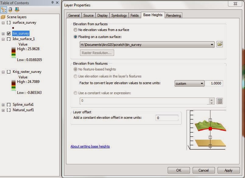Figure 3: Under the layer properties window in ArcScene, elevation values are able to be applied to a surface to allow 3D displays. By right clicking the layer in the table of contents then selecting properties, this window will appear and allow the user to assign these elevation values under the Base Heights tab. 

ArcScene Evaluation of Interpolation Rasters: ArcScene is capable of displaying the interpolations as 3D models. Open a new scene and add the new IDW, natural neighbor, spline, Kriging, and TIN rasters. The elevation values need to be set for each raster to have the display model the terrain. From the table of contents, right click a raster and select “Properties” from the drop down menu. Click the “BaseHeights” tab in the layer properties window (Figure 3). Under the “elevation from surfaces” box, click the “floating custom surface” bubble. In the drop down box, make sure the layer you are working with is selected, and then click apply and ok to close the window. The layer selected will now be displayed using the elevation values and model the surface. The same process can be done for each raster to display the elevation curves. Toggle the layers on and off to compare the interpolations.
   

Discussion/Revisit: Several interesting observations were made using the interpolation models, the first being the arrangement of the features. In all the models, the locations of the features were mirrored perfectly. The elevation values were correct the horizontal location of each was opposite of the real world terrain. Coordinate values were reviewed but were correctly entered into the system so the issue remains unresolved.

Figure 4: The Kriging interpolation of the terrain was the most realistic and representative of the snow surface. The left image is an aerial view of the interpolation results, while the right is a 3D representation of those results. Boundaries of features are smooth and gradual in transition to the surrounding elements mimicking the snow. 

Of the five types of interpolation methods, the Kriging method returned a model that best resembled the real world snow terrain in the planter box (Figure 4). Feature boundaries were smooth and gradual such as those in the terrain. The edges of the valley were not defined as well as the real world terrain but were represented correctly by the assigned values. The next best model was the spline interpolation (Figure 5). Like the Kriging, the feature boundaries molded into the plain but in the spline, small imperfections in the plain and along the edge of the valley differ from the snow terrain model.

Figure 5: Results of the different interpolations. The TIN (top left) surface is accurate in location of features but not in the structure of the features. Spline results (top right) display over the plain peaks where the survey points were located created a washboard effect over what is really a smooth surface. This is very similar to the IDW (bottom right) display that small peaks are shown in the model. Also the boundaries of the features are varied and not as continuous as the snow counter parts. The natural neighbor model (bottom left) is middle ground between the IDW and Spline. Feature edges are continuous but the surface is wash boarded from the imperfections in the interpolation. 

The TIN was accurate in its representation of the feature locations and general shapes, but the resolution of survey points was coarse (Figure 5). To create a more realistic model using a TIN, more survey points may have been taken around and of the snow features. The increased number of points usable by the tool would allow smaller triangles to shape the real world features more realistically. Natural neighbor interpolation was the worst in representing the real terrain (Figure 5). Along the flat plain surface, small peaks were created in the model where the survey points were. This created a washboard appearance to the model that was unrealistic. The ridge was less defined in elevation change from the plain as well as the boundaries of the other features. Edges of the features were not gradual and even throughout the model, falsely representing the snow surface.

        As in all field work, the field provided a few big challenges in this exercise. Wisconsin, after all, isn't known for gentle pleasant winters. With air temperatures hovering around 10 degrees Fahrenheit with wind chills below zero, dexterity became an issue. Not being able to feel or move your fingers makes any job harder especially one that requires patients and accuracy in measuring features you sculpted out of snow. Also with the temperatures being so cold, the moisture content of the snow was very low. For an example, try forming a ball from powder sugar. The light, fine, and fluffy snow made forming the ridges and peaks tricky. The features were soft and not as rigid as ones that could have been made from heavier snow. This made measuring difficult since the surfaces of the features weren't solid. We had to be careful not to alter the surfaces when moving the meter stick from cell to cell. Using the string allowed the measurements to be made without changing the faces of the features drastically since the string was able to mold around the surface but still hold true to location.

Conclusion: Field work is unpredictable. Each day, especially in Wisconsin, is its own identity in terms of weather and you have to plan for everything. Weather changes along with the availability of tools and supplies. Being able to solve problems with limited resources is a skill that is great in any situation not just field work. Having the persistence and the ability to work through and problem solve successfully in these types of situations demonstrates commitment and responsibility to an employer.