UAS Field Day 2 and 3

Introduction: Aerial imaging via unmanned aerial systems (UAS) is becoming more and more affordable to the public. Simple digital cameras can be mounted on a kite or balloon, set on a timer to take pictures at intervals, and launched into the air. Of course, more sophisticated systems can be built such as the Y6 shown earlier, but complexity and expense are only obstacles if you want them to be. This exercise involved capturing aerial imagery via balloon and Y6 rotocopter. Each resulting set of photographs were then mosaicked into an orthophoto using Agisoft Photoscan. In normal aerial photos, there is error caused by the angle the camera is taking the image or natural changes in the surface that is being imaged. An orthophoto is an image that has been geometrically correct to remove any error caused by buildings, large changes in the surface, or if the images were taken at an oblique angle. The orthophoto is to scale with the real world objects and scenes photographed where a normal image could be stretched in certain areas. This is important if the images are to be used in any sort of mapping done needing a distance calculation. Agisoft Photoscan is a modeling software that allows images to be loaded and built into an orthophoto and 3D surface based on a generated point cloud. The newly created orthophotos were then georeferenced to the surface imaged with the use of ArcMap.

Study Area: Eau Claire Indoor Sport Complex and Soccer Fields, Eau Claire, Wisconsin

Methods:

Y6 Rotocopter: The Y6 rotocopter is the more sophisticated of the two platforms used to image the area around the indoor sports center. The systems has the necessary autopilot software and stabilization systems to carry a digital camera for the imaging. A flight plan was programmed into the autopilot software and Canon- SX260 digital camera was set to take a still image every 2 seconds for the duration of the flight. The resulting photoset held about 500 pictures. Of those 500, 105 were chosen based on clarity and continuity to be mosaicked in Agisoft Photoscan. The resulting orthophoto was then added to the ArcMap document with a satellite base map. Because the GPS on the camera logged in WGS-84, the orthophoto was projected using the “project raster” tool in ArcMap to UTM Zone 15N. The now projected orthophoto was georeferenced to the satellite base map using the “Georeferencing toolbar” in ArcMap. To reference the photo, click the “add control points” button from the Georeferencing toolbar. Then click an area on the orthophoto, such as an intersection, to set a ground control point. Now find and click on the same point on the satellite image. The orthophoto will be stretched to match the points to the points on the satellite image. It helps adjust the orthophoto transparency to help see the satellite image below. After the orthophoto aligns with the satellite image, select “rectify” from the georeferencing menu on the toolbar. This will save the edits made when the image was matched to the satellite base map.

    

Balloon: The balloon was flown at a height of a couple hundred feet. From the tether string, a camera mount was strung and held a Canon-Elph110HS digital camera. The camera was set to snap a still image every 2-3 seconds for 20 minutes. From the picture set, 96 were chosen to mosaic in Agisoft Photoscan. Before mosaicking the images, the GPX track needed to be appended to the images. 

Figure 1: GeoSetter offers a platform that makes linking the GPX track log to the images captured. Having a GPS location with the image improves the accuracy of the later orthophoto.

To assign the GPS location for each image, the 96 images were imported into GeoSetter (Figure 1). By clicking the “synchronize with GPS data file” button on the toolbar, GeoSetter aligned the images with their proper location and saved each image with a GPS coordinate. Now that the images have a GPS location, Agisoft Photoscan can properly make the mosaic and orthophoto. The orthophoto was then added to the ArcMap project with the satellite base map. The image was projected using the “project raster” tool in ArcMap from WGS-84 to UTM Zone 15N. Then using the same process as before, the image was georeferenced to the satellite image via the georeferencing toolbar. To save the referenced image, select “rectify” from the georeference menu on the toolbar.

Figure 2: Agisoft Photoscan uses the selected images added in the workspace and creates a 3D model of the surface. The images are linked, allowing the creation of a point cloud which the program uses to model the real world surface. 

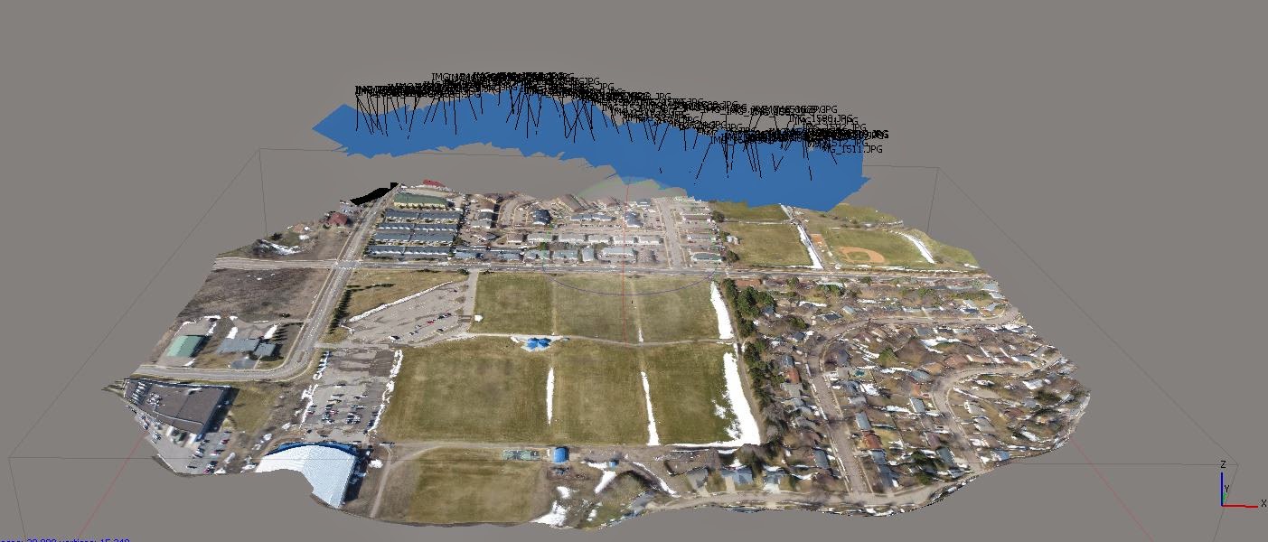
Orthomosaic: Agisoft Photoscan was used to create the orthophotos from the collected aerial images. From the workflow tab in Photoscan, select “add photos”. This will bring the photos that will be mosaicked into the workspace. Now from the workflow tab, select “align photos”. The program will form a point cloud using all the images selected in this step. If a high number of images is used, the processing time will take longer. With both platforms using about 100 images each, processing took about 15 minutes. From the newly created point cloud, select “build mesh” from the workflow tab. This creates a TIN from the point cloud turning the 2D images into a 3D surface (Figure 2). Now to add the imagery on top of the TIN, select “create texture” from the workflow tab. Once the texture is added, export the orthophoto from the file tab in a TIFF format to be imported in ArcMap for georeferencing.

Georeferencing: Open a new ArcMap project and add a satellite image base map and set the map projection to UTM Zone 15N. Add the orthophoto TIFF created from Agisoft Photoscan. Before referencing, use the “project raster” tool to project the TIFF from WGS-84 to UTM Zone 15N. This will make the referencing process a little simpler and more accurate. Now to start referencing, open the Georeferencing toolbar from the customize tab in ArcMap. On the toolbar, make sure the TIFF is listed in the drop down box and select “add reference points”. Using the tool, click an area on the TIFF and match that spot to that of the satellite base map. Change the transparency of the TIFF to about 30% to help locate features such as intersections or corners of buildings to help accuracy. Repeat this process of clicking the image, clicking the satellite base map until the image matches the base map. Once the image matches, select “rectify” from the georeferencing drop down menu on the toolbar. This will save a new image that will now be georeferenced.

   

Results:

Figure 3: The georeferenced (bottom) and original orthophoto (top) comparison show how georeferencing can have a big impact on scale of an area imaged.

Y6 Rotocopter: The resulting orthophoto from Photoscan was clear and representative of the survey area. It took 15 ground control points when georeferencing to match the orthophoto to the satellite image (Figure 3). The edges experienced the most distortion especially noticeable in the residential areas.

Figure 4: Comparison of before and after georeferencing for the balloon imagery. The bottom image is georeferenced where the top is still disoriented in space over the map. 

Balloon: The orthophoto created from the balloon imagery was too distorted more on the edges of the image than the interior. The image was referenced using 8 ground control points on the images. Although it took less points to correct the balloon image, there was more discrepancies originally than in the Y6 orthophoto.

Figure 5: The Y6 has a compensation rig that allows the digital camera, while engaged in photography, to remain parallel with the ground. This keeps distortion in images to a minimum regardless of wind conditions and keeps the camera in a stable position. 

Discussion: The Y6 imagery was finer and more defined than that of the balloon. This may have to do with how the camera was mounted to the platform. The setup on the Y6 was an electric gyroscope that had automatic compensation for changes in the camera angle (Figure 5). If a gust of wind came up, the system automatically kept the camera parallel to the ground. The balloon’s camera was mounted using string and a couple brackets purchased at your local hardware store for under 5$. The rig kept the camera level but there was no way to compensate for wind gusts since it was attached directly to the string of the balloon. The Y6 camera also had the ability to automatically geotag each image collected during the flight. The balloon images had to later be processed using the GeoSetter software to link the GPX file captured on the rig to the images collected in the same location. If the balloon images were mosaicked without geotagging the images, the resulting orthophoto was displayed off the west coast of the Galapagos Islands in ArcMap, even after the correct projection had been defined. 

Figure 6: Without geotagging the balloon imagery before mosaicking, even with the defined projection, the orthophoto is displayed off the coast of the Galapagos Islands (red circle) instead of over Eau Claire, WI (green circle)

Even with the automatic tagging for the GPS locations, the cameras collect in WGS-84. It is important to remember this to correct the projections before you georeference it. The varying displays from different projections by the satellite base map could distort the accuracy of the referencing. Overall the Y6 performed more reliably but this exercise proves that even with a low budget, it’s possible to collect suitable aerial images to help map and survey locations.

Navigation 3: GPS and Map Race

Introduction: Navigation with GPS systems has definitely become more mainstream with the option of dashboard systems. Most new vehicles today have options for turn-by-turn navigation giving the appearance that GPS systems are rarely wrong. GPS systems in vehicles are more reliable than handheld systems but still need to be used with common sense. Handheld systems are dependent on strong satellite signals. With weak signal due to cloud cover, dense vegetation, or tall structures, accuracy can be very limited. When navigating with a GPS, it is always good practice to have a map also as a reference in cases of low satellite signal or lost signal. For this navigation exercise, a Juno GPS unit and a map were used to navigate all 15 points of the Priory Navigation Course. To add a little incentive, the team who completed the course first received a prize, but all teams were armed with paintball markers. If a team member was hit with a paintball, a 30 second penalty was instituted.

Methods: Using the Priory geodatabase from Dr. Hupy and the maps created for the map and compass exercise, a new base map with all 15 navigation points of the course were added. Then using the digital elevation model provided in the geodatabase, the “slope” tool was used to find areas where the topography had the highest change in slope degree. Being a race, the group wanted to avoid running up and down steep slopes through the woods instead of find the points below and on top of the slopes first. The output feature class of the slope tool was then reclassified using the “reclassify” tool. This allowed areas with similar degrees in the slope to be grouped together and symbolized. The 10  default classes were simplified to 3: high, moderate, and low (Figure 1).  

Figure 1: The slope reclassification from low (green) to high (red) degree is displayed at 70% transparency under the planned path of travel. The starting point (5) was assigned but from there, the path was determined both by nearest point and the path of least resistance either slope change or knowledge of vegetation type. 

After we identified where the areas of the highest sloping terrain were and how to avoid them, we plotted our path starting at the assigned “point 5”.  To test the accuracy of the reported locations of the 15 navigation points, each team had to collect GPS data for every point they reached. In the map document in ArcGIS, an empty point feature class was created to hold the collect GPS points. This feature class needed a point number field, and our group chose to set a domain to restrict the accepted values to 0-15 since there were only 15 possible points. The path, navigation course points, and empty point feature class were then deployed to a Juno GPS which was used as a guide when running the course at the Priory. A paper map was also printed. The reclassified slope feature class, point feature class, navigation path, large Priory paths, and no shooting zones were included to help monitor progress and aid in navigation when GPS strength was low. As an added attribute field for the path feature class, the pace count from each point to the next was calculated in ArcGIS. Right click on the new field in the attribute table and select "calculate field" from the drop down menu. Using the “shape_length” field in the path attribute table, the new pace field was calculated by (shape_length)*(64/100) since the pace count in 100 meters was 64 (Figure 2).  By having each pace count listed on the side of the paper map, this saved time trying to calculate each in the field and still gave a reference on how far we were to travel.

Figure 2: After the new "pace" field was added to the path feature class, the field was calculated with the expression shown above. The shape_length field automatically calculated by ArcGIS was used as a base distance from point to point, then the pace count in 100 meters was used to convert that point-to-point distance to a pace distance. 

Results: Our team navigated the 15 point course in about an hour and a half resulting in a second place finish. The GPS display was helpful to keep on path and the calculated pace count helped keep us within the correct distances. The collected GPS points by the team matched the original navigation points fairly well with the exception of 7, 11, 14, and 15 (Figure 3). Using the measuring tool in ArcGIS, the points collected by the team were measured at most 15 meters different from those reported.  

Figure 3: The collected GPS points are represented by the orange boxes and original point locations are represented by the red circles. Points that were the most different were those in locations with dense vegetation or high variation in slope values. 

Discussion:  

Navigation: The path created by the team worked fairly well in the field. The first half, from points 5 to 3, were all found with little exertion from walking through the woods; however, points 3 to 1 were located in terrain that held gullies and high ridges that were unavoidable. Having this at the end of the course was probably not the best idea, but since we were assigned point 5 to begin we really had no choice.  Point 2 was the hardest location to collect since it was down in the bottom of a steep, deep gully (Figure 1). Obviously the high ground is the place to be in a fire fight, so we nominated a single team member to run down with the Juno to collect the point. No casualties resulted.

Paintball Gear: Carrying a paintball marker while wearing a mask that is fogged up isn’t the easiest way to navigate a course like this. The markers were heavy since the hoppers were high above the top of the marker and the air tanks were bulky in the back. The masks were hot and fogged up after a while, making readability of the map and GPS difficult and walking through the course. The fog also effected how well you were able to see other teams to avoid getting hit and serving the 30 second time penalty. You also had to be fairly close to the opposing team during fire fights to be able to hit them. The trajectory of the paintballs was fairly erratic making accuracy only a wish. The masks weren’t all bad though. They did help by protecting your face from branches and buckthorn while walking through a few of the dense areas of vegetation. 

Juno GPS: The GPS units did make traveling and navigating the course quicker than just the map and compass as previously used. The visual display of the route the group was traveling with the display of our current location allowed us to travel and adjust accordingly to stay on course. When navigating using compass bearing, once you are off the line from point to point, it is difficult to arrive in the correct location to find the navigation point in question. The Juno wasn’t perfect however. Several times, 4, we had to reset the system due to bad satellite signal or hitting a button while running through the woods or shooting our paintball markers at a rival team. The satellite signal could also have contributed to the variation in the point location noted earlier. The points that displayed the largest discrepancy were those in areas where the terrain varied more so than the surrounding areas and the vegetation was dense (Figure 3). The trees, although still without leaves, create an obstacle for satellite signals to be received through making the accuracy of the GPS limited. Also, to reduce the display time for the GPS, we removed the base map from the display. Without having the GPS draw the image each time we moved, this saved display time however we were more dependent on the paper map for reference, which isn’t a bad thing. Carrying the Juno also was a bulky nuisance at times. Between trying to track the path our team was taking to the next point and watch for rival teams, the GPS became a vulnerability. 

Navigation 2: Map and Compass Orienteering

Introduction: Map and compass navigation has been around for centuries and is the most tried and true form of navigation today. Without the need for a satellite signal, an adventurer can successfully navigate series checkpoints in all types of terrain and land cover. Adventure racing is a new and upcoming outdoor recreation that encompasses hiking/trekking, kayaking, mountain biking, navigation, and running into one cross-country race. No GPS technology is allowed other than a tracker provided by the event planners. The only form of navigation is a map and compass. Being able to quickly map, measure, and locate each checkpoint allows an adventure team to be successful and win the races. For our purposes, we were navigating 6 points in one very local area, where these adventure races can hold hundreds of checkpoints and span several countries. Compass navigation is a simple but very powerful skill set to have in your day to day life.    

Study Area: The Priory, formerly known as St. Bede’s Monastery, was purchased by the UW-Eau Claire Foundation in 2011. The 3-building complex and 112 acres were used as an education facility for the Sisters, and is today home to the Children’s Center and Nature Academy. The UWEC foundation is leasing the land to the University of Wisconsin – Eau Claire which also uses the living quarters as an extension of the residence halls for college students. The surrounding acreage is currently used for nature hikes and a 15 point orienteering course (Figure 1).

Figure 1:  Each of the 15 points of the adventure course on the Priory property are marked by orange and white flags with both numbers and unique hole punchers. There are cards given to each team with a grid to punch at each site.

Community discussions have recently been held on how to further the use of the land surrounding the complex. Ideas discussed include: community gardens, pollinator habitat, use as an outdoor classroom, and many others. The area is mostly oak forest but the lot also holds a large jack pine barren. The building complex is perched atop a plateau while the forests are in the surrounding lowland areas. A small holding pond for the waste water produced by the Priory is also on the property.      

Methods:

Figure 2: The 6 points assigned were plotted on the map using the grid system. Each point was then connected to allow for distances and pace counts to then be calculated. 

Plotting Point Locations: Before heading off into the woods, you need to know where your destinations are. A list of the point location coordinates was provided by Dr. Hupy. Depending on which coordinate system (UTM or Degrees Minutes Seconds) you are going to use, the corresponding point locations needed to be drawn on the map. Using the maps created in the first navigation exercise, the 6 selected points of the 15-point course were plotted using the grid system (Figure 2). The X coordinate is the Longitude so the x-axis of the grid was used to find the horizontal position. Once the x-position was found, the y-coordinate was used to plot the point location. Like the x, the Y-coordinate or latitude of the point location was found using the y-axis of the grid on the map.

Figure 3: Before heading into the woods, the bearing to the location was calculated using the drawn lines and the compass. By using the bearing from the map, the navigator can keep the group in line with the point when traveling through the woods. 

Navigating the course:  The next task was to determine the direction of travel, or bearing, to reach the first point from start. First, a line was drawn to connect the 2 points. Using this line, the compass was laid on the map along this line so the direction arrow was pointing to the destination. Then the bezel or dial on the compass was rotated to align the guidelines on the dial with the North South grid lines on the map (Figure 3). The degree reading aligned with the direction of travel arrow is now the bearing. To reach the point, the navigator turned their body to place the red north arrow in the red “shed” on the dial face of the compass. The pacer determined the distance to the point by converting the map distance to real-world pace determined in the previous navigation exercise. With the bearing and distance now known, the navigator sent the runner out ahead of the pacer. The runner allowed the navigator to line up a path for the pacer to help make counting pace more manageable. Once the pacer reached the calculated distance, the point in question should be within sight distance IF the runner and pacer stayed on line with the navigator’s bearing. After the first point was reached, the same process was repeated to reach the following 5.   

Figure 4: Terrain and vegetation varied across the course from thick under brush in the oak forests (left) to the open pine barrens (right). Depending on what we were traveling and navigating through, the pace counts needed to be altered to compensate.

Results/Discussion: The group overall navigated the 6-point mini course in about an hour and 45 minutes. With the 3-person navigator, pacer, runner scheme it was quick work once a rhythm was established. The points assigned to us were over a variety of terrain and land cover ranging from dense oak forest, pine barren (Figure 4), to open field and relatively flat to deep steep ravines. The third point, point “8”, on the map was located about 50 meters south of the real world location. This lead the next point’s bearing to be off from our map and the group actually overshot the location for point 9 (Figure 5).

Figure 5: Point 8 (left) was given different coordinates than the real world location. The red circle displays the area where the point was actually located. This created problems when navigating to point 9 (right). The group overshot the location and used the intersection noted by the red circle to take a new bearing to point 9.

Using a land mark, the intersection of two roads, a new bearing to the plotted point location for 9 was taken, leading to the real location (Figure 5). The following points, 10,11, were found without any problems. The terrain was difficult to see through, meaning the runner had to keep relatively close for the pacer to see and travel (Figure 6). The thick underbrush also meant having to add several paces onto the calculated values since a direct path wasn’t always an option to travel. It is important to not set the runner too far ahead since the increased distance opens up the possibility of straying from the bearing. If traveling a large distance, the more precise or true to your bearing, the better luck you will have finding the destination.

Figure 6: Steep terrain and thick under brush of briers made visibility and traveling interesting in sections between points 8 and 9.

Terrain Surveying with a TOPCON Total Station

Introduction: In more critical and precise applications, a total station can be used to survey the surface of an area. The total station uses both distance and azimuth as well as an elevation to record and plot the points selected by the operators. The base stations location is plotted using a GPS receiver. Using that location as a reference, points in the survey area are captured using a laser and reflective prism by the base station. The base station emits a laser that hits the prism at the point location, then relays the information via Bluetooth to the GPS receiver. The distance to that point is recorded and automatically calculated into an x, y, z position based again on the base station’s original GPS location and the use of a backsight. The backsight provides the base station a reference to north. Without this reference, the points would only be relative to that single base station location and not real world location. In this exercise, a 1 hectare section of the University of Wisconsin-Eau Claire campus mall was to be surveyed to capture the micro-topography. A TOPCON GTS-250 series total station with GMS-2 receiver were used to collect the positions and elevation data from the hectare plot.

Figure 1: The new UW-Eau Claire campus mall was formerly the home of the old Davies Student Center. Now the space is used as a seating and performance area for campus events. 

Study Area: The campus mall of the University of Wisconsin-Eau Claire has undergone major construction in the last couple years. The area was previously occupied by the old Davies student center but now is a new green space with seating and performance areas. This opened up the center of campus for different events provided by the University’s numerous organizations (Figure 1). The seating area is a miniature amphitheater with a gentle slope down to the new brick staging area.

Methods:

Figure 2: When setting up the total station, one has to step with care around the legs of the tripod. This prevents the legs from settling more after the station is leveled. By course then fine adjusting the level using the legs, fine adjustment is quicker and easier with the adjustment knobs at the base of the total station. 

        Setting up: Before starting to collect data, the survey plot and base station need to be properly setup. The survey hectare was measured using a pace count. Since a hectare is 100 x 100 meters, the pace counts measured in the previous navigation exercise was applied. The pacer placed a flag at each corner of the survey area. This provided a rough measurement for what area needed to be captured using the total station. With the hectare now set, a location for the base station was selected. The tripod was then set and secured over that location. When setting up the tripod and total station, it is important to make sure that the legs of the tripod are wide enough to provide stability and the tripod is at a comfortable height to work with (Figure 2). Using the level on the tripod, the station was “rough” leveled then more precisely leveled using the fine adjustment tools on the TOPCON station. Once the station was level, the GPS location and backsight information can be set. It is important to check to make sure the Bluetooth is enabled on both the station and the receiver. The settings – parameters menu on the total station allows you to turn the Bluetooth on. The “B” icon will the visible on the home screen once the Bluetooth is connected to the receiver. Now using the GMS-2 receiver, the base station GPS location was collected. The averaged location named “OCC1” for occupied point 1 was then able to be selected from a list to be assigned as the base station’s location in the TOPSURV software on the GMS-2. Next was to set the backsight in the observation – total station menu. Using a land mark and flag, the azimuth from the base station to the point was measured. A TruPulse laser range finder provided a precise azimuth which was then set as the default backsight on the station. Since the goal of the exercise was to capture the micro-topography, it is also important to set a base height for the station and prism rod. Using a measuring tape and the designated mark on the TOPCON station, the height was measured then set in the menu. The height of the prism rod is marked on the rod itself which was kept at 2 meters.

        Data Collection: Before evening thinking about collecting points, make sure that the black locking knobs on the total station are facing away from the viewing lens. If they are on the same side you are working on, the station will not allow you to collect any data points. Now that is cleared up, the surface data can be collected. The rod operator will walk out to the corner of the hectare plot and hold the prism level facing the total station. The total station operator will then align the view finder cross hairs with the prism rod and collects the point with the GMS-2. Once the GMS-2 notifies that the point has been collected, the rod operator will move and the collection process with repeat. The area was surveyed at 6-7 pace intervals between collection points.

Figure 3: The data exported from the GMS-2 to a text file result in this form. The point name, y location, x location, and z locations are listed from left to right. When opening the text file in Excel, make sure to select the comma as the deliminator and not the default tab setting. This will keep each set of information values in their own columns, x in one, y in another and so on. 

        Exporting the Data: From the job menu on the GMS-2, select export – to file. Choose points and export as a text file. The text file keeps the x, y, and z information (Figure 3). If the file is exported as a shapefile, just the locations will be kept without the assigned x, y, and z coordinates. Without the coordinates, just the points would be able to be mapped not the surface model. Once the text file is created, transfer the file from the GMS-2 to the computer with Active Sync.

        Creating the Surface model: The new text file created from the GMS-2 was opened in Microsoft Excel. In the dialog box, make sure that the comma is used as the deliminator and NOT tab. The column headings were checked to ensure that the correct data values were listed. In the text file, the X and Y values were switched and needed to be labeled properly before the excel table was saved. Next the excel table with the point values was imported into ArcScene. This process is the same as described in the previous “Terrain Survey” exercise. Right click “Layers” under the table of contents. From the menu select “add data” and browse to find the excel table. Once the table has been added to the layer, right click the table and select “display xy data” from the menu. The default values will be set in the dialog box so verify that the x, y, and z values are all correctly assigned and selected to be displayed. Once the points are displayed in the map area, the feature class can be exported to save the display values with each point position. Without exporting the feature class, the individual point values are lost. Now using the point feature class, interpolation to create the surface model was completed. Based on the results from the interpolation methods explored in the previous “terrain survey” exercise, the Kriging interpolation was chosen to create the surface model. The Kriging interpolation was performed by running the “Kriging” tool from the ArcGIS toolbox. To run the tool, open ArcToolbox and expand the “3D analysis tools” toolset. From the “Raster Interpolation” toolset, select “Kriging”. The tool window will open. Use the point feature class as the “input features”. Make sure to select the Z field as the “Z value field” to make sure the tool uses the elevation values in the interpolation. Name the output raster, accept the all the default values, and select OK to run the interpolation.

Figure 4: The collected survey points were used to create a surface via Kriging interpolation. The occupy point, or location of the total station, is represented by the blue dot towards the center of the surface. Areas with larger changes in elevation were surveyed at higher point densities. This can be seen in the low lying area around what is Little Niagara Creek. 

Results/Discussion: The surface model generated by the Kriging interpolation did represent the real world surface of the UW-Eau Claire campus mall (Figure 4). Because the grade or slope of the hectare was gradual, there isn’t a drastic change in elevation which is mimicked in the model (Figure 5). The areas where the slope was steeper, more survey points were collected. This is demonstrated by the area surrounding the Little Niagara Creek. The banks of the creek were in the low-lying area of the mall, therefore the surrounding approach to the creek displayed most of the elevation change over the hectare.

Figure 5: The profile of the interpolated surface is relatively accurate to the real world area surveyed. The campus green space gradually slopes to the creek with seating on the slopes. The slope levels out towards the base of the creek due to a staging area for campus events. 

As noted before, we first had a problem with collecting survey points due to the locking knobs on the total station being on the same side we were viewing from. Once we rotated the view finder around to the other side, the points were able to be collected successfully. When importing the text file, the x and y coordinates were listed in y, x order. The table needed to be labeled properly before added to the map document in ArcScene. If the columns weren’t labeled it is quite possible to assign the wrong values to the x, y and z fields when displaying the data. This would result in a misrepresentation of the surveyed hectare on the mall.

Conclusion: The use of a total station when surveying a terrain is a very powerful tool, but the accuracy of the survey is only that of the GPS used to record the data. Because the location of the total station is used to reference all other measured points, the accuracy of that first point determines the accuracy of all the later collected data. The degree and precision at which the station collects data is extremely high regardless. The laser and prism allows the station to report high accuracy data points even if the prism rod is hundreds of feet or meters away from the station. This was not the case with TruPulse range finder which was used in the previous distance azimuth survey. The ability for the station to collect and automatically correct the data for x, y, and z positioning is a great feature to save computing and data prepping time.

UAS Field Day: 1

Unmanned aerial systems (UAS) are becoming more and more common place in the general public. Model rockets, helicopter kits, balloons, and even kites are possible systems to which a camera or sensor can be attached. Imagery (with some computer software processing) can be collected using low budget UAS and still be reliable to the user. Like all GIS projects, what the topic of interest and the area needed to survey determines how you will need to collect data. The images below are a few of the systems the class was able to see demonstrated at the soccer fields by the Eau Claire Indoor Sports Center. Plus, who doesn't like to be outside on a 60° day after a brutal Wisconsin winter in Eau Claire, WI.

Equipment:

Figure 1 (left) and 2 (right): In a multidisciplinary research venture between the geography and physics departments of UW-Eau Claire, the design and functionality of a roto-copter UAS was demonstrated for the geospatial field methods class. Both maneuverability and autopilot software were demonstrated in the 20 minute flight time.  

Figure 3 (left) and 4 (right): Roto-copters have several setup options. The figure 3 copter is the one designed by the joint research effort through UW-Eau Claire and the figure 4 copter is owned by Dr. Hupy. Dr. Hupy's copter is fitted with a gyroscope mount for a digital camera. This allows the camera to remain level to photograph while the copter is banking or turning to compensate for win or flight plans. 

Figure 5: A side-by-side comparison of the research copter (left) and Dr. Hupy's copter (right/back).  The research copter has 6 arms but only single bladed. Dr. Hupy's only has 3 arms but has double blades, one on the top and one on the underside of each arm. Depending on what the payload and flying conditions are, either setup could be beneficial. 

Figure 6 (left) and 7 (right): UAS aren't all high cost. Something as simple as a kite can capture images from the air on a small budget. This kite is 8 feet wide and as long as there's a steady wind, provides a stable option for aerial photos.

Figure 8 (left) and 9 (right): For this demonstration, a digital camera was attached to the kite string using less than 5$ worth of hardware supplies. A couple clips to wrap the kite string around, 2 flat mounting brackets, and some string is all it takes to built a digital camera sling. 

Figures 10 and 11: Once the digital camera is secure to the kite string, the kite string is let out to allow the camera to be carried high into the air. By setting the camera to take pictures in a set interval for a determined duration, all you have to worry about it flying the kite. We let about 300ft worth of string out for the kite.

Figure 12 and 13: Another type of UAS is a rocket. Model rockets come is single, double, or even triple stages. The stage determines how many engines the rocket can hold. The rocket shown is 2 stages, meaning it holds 2 engines. The first will be ignited by the electric ignition box, then the second will be ignited by the end burst of the first engine. We attached a small video camera to the body tube to record the flight from the sky. 

      Camera Results:

Figure 14: The photos above are still shots captured by the Cannon digital camera that we suspended from the kite. Even with the wind blowing strong, the kite provided a nice, stable positing for the camera to take clear photos of the surrounding area. 

Figure 15: This is the video captured by the small camera we attached to the rocket. Only the first stage fired correctly, but still made for an entertaining minute to watch. 

Database Creation for Micro-Climate Mapping

When starting a geospatial project, it is import to consider exactly what data you are going to be collecting for the project before you venture off into the field. By planning an organized geodatabase, the data collected from the field can be imported into ArcGIS in a more user friendly manner. In this GIS exercise, a geodatabase will be created to hold data about micro-climates around the University of Wisconsin-Eau Claire campus.

 How can a geodatabase be used in the field?

 New hand-held GPS units are becoming portable computers. A user can create feature classes and log data directly into a database out in the field without needing a full version of ArcGIS. These features, however convenient they seem now, can be a double edged sword. If multiple feature classes are created “on the fly” in the field, data are separated into those separate feature classes. If the user considers what they want to record for data before leaving the lab to the site, all the data can be logged into a singular feature class. Creating feature classes out in the field also can lead to input data errors which can misrepresent information, costing more time in the future. Using a singular feature class that holds all the attributes one wishes to record in the field, stores all the information for each location together instead of separate feature classes. Separate classes open the possibility that data may be assigned to wrong locations or may be forgotten and not recorded. Also, by planning the geodatabase beforehand, all fields or attributes collected, can be assigned a range or code to help eliminate data entry errors to help improve the data integrity. These ranges or coded values are Domains. Domains ranges or codes can be applied to a field so only values that fall in that range or assigned code are allowed to be recorded into the feature class. The same domain may be set to multiple fields if those fields have the same data range or codes. Domains can also be associated with all different field types available in a feature class, which include: short integer (short), long integer (long), single precision floating point numbers (float), double precision floating point numbers (double), alphanumeric characters (text), data and time data (date). When assigning the domains, only those that match the field type of the field in question will be available to assign. This will be demonstrated below. As domains are created for the fields, they are saved inside the geodatabase and can be accessed or edited throughout the project. With all the domains set to the fields created in the single feature class, when the database is loaded onto the portable unit, data entry will be faster and more accurate for analysis later.

Using a Geodatabase in Microclimate mapping: What information needs to be collected?

• ·         Temperature
• ·         Dew point
• ·         Wind speed/direction
• ·         Snow depth
• ·         Relative Humidity
• ·         Time
• ·         Notes of the surrounding area  

 

Figure 1: From the geodatabase properties menu, two tabs are displayed. The domains are created here with all descriptions, codes, and ranges to later be assigned to feature class fields. 

Domains: To create new domains for use in feature classes, right click on the geodatabase and select properties. A new window will open having two tabs: general and domains (Figure 1). The domain tab is where you can name and assign parameters for each field you wish to collect. For the information listed above, the following domains were created:

• ·         Temperature – Float, type: range, minimum 0 maximum 99
• ·         Dew point – Float, range, 0-100
• ·         Wind speed/direction – float, range, 0-360
• ·         Snow depth – float, range, 0-36
• ·         Relative Humidity – float, range, 0-100
• ·         Time – short integer, range, 0-2400
• ·         Notes of the surrounding area – Text

Once all the needed domains are created, click OK. The domains will now be listed in the property field when created fields for a new feature class. Only those domains that match the data type for a field will be listed in the menu.     

Figure 2: The feature class properties will display all fields listed in the feature class along with any set parameters such as domains. 

Feature classes: For this project, each spot surveyed for microclimate data are going to be saved as a point feature. Since multiple features can be linked to a single point, it’s best to use a single feature class with multiple fields. Each piece of information listed above will have its own field in the feature class (Figure 2). To create a feature class right click on the file geodatabase you wish to add the data to. Then select new-feature class. A new window will open leading you through the process of creating the new feature class. 

Figure 3: When creating a new feature class in a geodatabase, a new window will open. Follow the prompts to define the projection then at this window the fields will be created. Each field has an assigned data type and domain associated with what is being collected.

You will first name and assign a coordinate system, then proceed to the window that prompts for field names and data types (Figure 3). This is where you will add the field title for each piece of data collected. The data type will depend on the field and can be text or numeric. Here is also where you will assign the domains created before to each field. In the Field properties box, click the area next to “Domain”. This will have a drop down box where you will be able to select the correct domain for each field in the feature class. Once all the fields are created and domains assigned, click finish to setup the feature class.

Navigation Part 1: Map Construction and Bearing Navigation

Introduction: The use of a compass as a tool to navigate the globe has spanned centuries. Without a good compass and map, sailors wouldn’t have been able to navigate seas limiting the extent of trade and expansion. The ability to use these tools to navigate has become somewhat of a lost art so to speak with the invention of global position systems or GPS. A location can be digitally entered and saved into these systems and the device will navigate the user to those logged locations; however, without the use of a map too, the path a user would travel may not be the most direct or advantageous. GPS also requires a strong satellite signal to operate with relative accuracy which isn’t always possible in dense vegetation or terrain one might find themselves in. This is where the simple compass beats out the fancy bells and whistles of GPS. Using a map and the bearings or directions of travel from a compass, one can successfully navigate as well or even better than a GPS. This exercise will demonstrate the time-tested method of compass navigation.

  

Maps: A navigator is only as good as their map. If the map representation of the area one wishes to navigate is incorrect, there is little chance that even with GPS navigation would be successful. For this exercise, we created our own maps as tools for later navigation races. The area where our navigation course is set up is called The Priory and is owned by the University of Wisconsin – Eau Claire Foundation. The Priory is 112 acres and is the home of a former monastery. The University foundation purchased and leased the land and structures to the University of Wisconsin – Eau Claire to provide a location for the Children’s Nature Academy and use the housing as a new resident hall for students. The area is mostly forested with stark topography created by the prehistoric ridge. Since the location wanting to navigate is local, a large scale map is best requiring a coordinate system and projection that has a high level of accuracy for these scales. It is also important to identify what information is necessary and what is noise. A navigation map needs to have essentials such as topography to see if in any mountains will be crossed in a path from point to point and several landmarks that a navigator can use as a reference. If the map is too busy or noisy, navigation is more difficult since the map is hard to read. You want to be able to quickly understand and find relatively where you are situated rather than spend hours just trying to find where you started. Data including a 5-meter topography and navigation boundary were acquired from a prepared database by the instructor Joe Hupy. A topography of an area could be acquired by using a 15-minute topographic map that is produced by the United States Geological Survey (USGS). The background satellite image was added in ArcMap using ESRI basemap datasets.  

Methods: 

Map Creation in ESRI ArcMap: As mentioned above, coordinate system and projection are the most important aspect to consider when creating a map. The local, large scale needed for a navigation map of The Priory required the accuracy and usability of a specific projection. The geographic coordinate system for North America updated in 1983 provided the base for the necessary projection. Using the North American Datum 1983 (NAD 83) Wisconsin Transverse Mercator projected allowed for the local level accuracy required. The state system provides better real world accuracy than just leaving the projection at NAD 83 since more local survey points were logged and referenced.

Figure 1: A navigation map including 5 meter topography and an aerial image background for the Priory was created using ESRI ArcMap. A measured grid displaying in UTM is overlaid to aid in locating destination points. 

The map units of meters also helps monitor traveling distance in the calculations later to come when planning a route. Now that the projection was chosen, the data were added. An ESRI aerial image base map was used as the background but was set to 70% transparency to keep the map readable but still be able to use the image as a reference. The navigation boundary, structure boundaries, and 5-meter topography provided from the prepared database were then added over the image. Like the aerial image, the structure boundary feature class was also displayed at a 50% transparency to reduce map noise. The topography class was also displayed with the elevation labels to keep slopes orientated in the field with those on the map (Figure 1). For plotting the destinations, a graticule and map grid were created to assist in the accuracy of the locations.

Figure 2: This is the same navigation map created before only is displayed using a decimal degree grid overlay. The decimal degree reference lines will aid in plotting points reported in degrees, minute, seconds or just decimal degrees.

Like mapping on a graph, the grids are used as a reference to help locate the positions or coordinates for the destinations and used to help determine the distance to those destinations. A grid using the Universal Transverse Mercator (UTM) measurements was added to plot locations given in meters or other UTM measurements (Figure 1) and another grid or graticule was added to help plot points given in decimal degrees from the Geographic Coordinate System (GCS) (Figure 2). The UTM grid lines always run vertically on the map regardless of where true north lies. This doesn’t always provide accurate locations for point destinations but at this large scale, won’t impact results greatly. Unlike the UTM grid, the GCS grid lines follow true north so are not vertical but are skewed to reflect the declination for the Priory location. This can provide better point locations when using a compass but, again, at this large scale, the discrepancies between UTM and GCS are minimized. The scale and representative fraction for the map were assigned and added by ArcMap. These are crucial in navigation as described shortly.

The Compass: The compass is an incredibly simple yet powerful tool. Compass navigation or orienteering is simple with a little bit of practice and knowledge of the compass itself. The most obvious feature is the bezel. The bezel is the rotating dial that holds the marked degree hashes used to determine bearings or direction you wish to travel. In the middle of the bezel you will find the needle as well as several index lines that will be explained in the Navigation section. The top of the compass has an arrow pointing away from the bezel this is your direction of travel. To use a compass, it has to be held flat in one’s hand parallel to the ground to allow the needle to rotate freely, and it is important to remember to keep the compass away from metal objects such as zippers in a jacket or a ring on your hand. The metal can affect the bearing from the needle. The needle has a red point and white point. The red always points to North therefore the white always to the South. The adage “keep red in the shed” refers to keeping the red north point in the designated red “shed” marked on the bezel. This is important for keeping the correct bearing when traveling.    

Navigation: First task to complete when navigating on foot is to determine a pace count. A pace is counted when a person is walking and the same foot is set on the ground, so for example 4 normal steps are actually 2 paces. For the later navigation, my pace count was 64 paces in 100 meters. Each person’s pace will be unique, so if you are going to count with a friend, don’t worry if you get different results. When pacing, it is important to try to take as normal sized steps as possible since this is how you will be walking on trails or through the woods. Depending on the terrain you wish to navigate, an addition of 20 or more paces may be necessary if steep slopes are going to be crossed. So after determining a pace count the next task is to plot your destination points on the maps. If the destination coordinates are known, a user can reference the grid or graticule that was added to the map to help accurately position the points on the map. If the coordinates are unknown but the destination is a landform, that’s okay too you can still use the compass to travel successfully. Not only do you have to know the destinations but also the starting location. This will be the first point where you will have to use a bearing and distance. Once all the points are plotted on the map, the compass can determine the bearings. To assign bearings, first draw a line connecting the starting point and the first destination point. Then place the compass side along the drawn line making sure the direction of travel arrow is indeed pointing toward the destination and turn the bezel to line the index lines inside up with the North and South grid lines on the map. The number or degree now lining up with the mark with the direction of travel arrow is the bearing to follow when traveling. When moving toward your destination you have to be careful to keep “red in the shed”. This is easier to accomplish if you choose objects or features that are in the line of travel and pace to them and check your bearing. By splitting the distance into chunks it helps to stay on line and not stray resulting in a different destination. BUT WAIT! Don’t head off into the woods yet, you need to know how far to walk! Measure the draw line between the starting and destination points, then using the map scale or representative fraction, figure how long the path is in real distance. Once you have the real world distance, convert that number into paces using your pace count. So if a map’s representative fraction is 1:100, 1 meter on the map would be 100 meters in the real world. This would mean a distance measured to be 250 meters would actually be 25,000 meters. Then using the pace count, 64 in 100 meters in my case, determine the real world pace count, 64*(25,000/100). So I would travel 16,000 paces if the topography was relatively flat. Remember if steep slopes are in the path of travel, additional paces should be added to compensate for the smaller step size. The generic equation for distance to pace is PACE*(REAL WORLD DISTANCE/ PACED DISTANCE). As explained earlier, not only is finding closer features that are on line better to follow a bearing but it also helps to break up the pace count since counting to 16,000 isn’t the easiest to remember when you’re wandering through the woods. When using features, just remember to log how many paces it was to that feature then subtract it from the initial pace count needed to reach your destination.